Team 1 Progress Report 4/7 Part 2

We have been making progress as a whole, both in the close reading essay and the search and comparison of the ad texts using digital tools.

Daniel’s initial findings through Voyant-

Initial searches of the Arkansas ads did not yield huge amounts of information, but enough to demonstrate that Voyant as a tool can help answer questions about the data.  Some of the use for Voyant can simply be demonstrating a lack of a strong trend on a certain topic.  The first question I used Voyant to answer was whether or not Texas slaves appeared to be receiving greater abuses or punishments than those in Arkansas.  This required a search for vocabulary sets related to this.  The close reading revealed that “scar”, “disfigure” and “lame” were used to describe slaves who seemed to have suffered injuries.  While there are many specifically listed injuries, those are the most frequently used.  By searching these words in all the sets of ads, I was able to reveal that Arkansas seemed to have proportionally more references to scars than Texas.

In our previous readings, we had talked about how slaves could have been more likely to have carried guns in dangerous Texas locations.  Searching the text for references to armed runaways carrying rifles, shotguns, or knives, I found the results to indicate that there were proportionally less references to guns in Texas than in Arkansas.

Searching for references to Mexico and Mexicans, I found nothing in the Arkansas ads referencing Mexico.  It does seem to be a Texas-specific location so far in terms of a destination for runaways.

There were proportionately more references to horses and mares in the Texas ads.  This could tie into the sheer size of Texas for escaping across, a higher likelihood of property owners having horses, or perhaps that the acquisition of horses was necessary to try to make it all the way to Mexico.

From the first search through the ads, there were a few specific improvements I had in mind for future searches.  One is to make a simpler way to compare numbers in data sets of different sizes.  I was using rough proportions to compare the quantities of occurrences, but somehow finding specific sets within the States that were the same size would make a more straightforward process.

Another issue is the inclusion of jailor’s ads.  For references to weapons and means of transportation, these will not be included as frequently in the ads of those already captured.  Thus, different proportions of included jailors ads in the sets will further skew results.

Future searches include terms describing the intelligence of slaves and descriptions of their skilled labor, to be compared to negative terms, as well as searches for references to accomplices, thieves, or others who might have persuaded or forced slaves to escape.

Geography Team Progress Report 4/7

Upon getting to work and trying to follow our schedule, we have realized that we planned to have too many things due in a very short period of time. We are in the process of adjusting the schedule and replanning what needs to be done. However, the three of us have been working on a few different tasks during the break.

Clare has been working on a draft of the close reading. Her rough draft includes an introduction, analysis of Arkansas, discussion of the advantages of the digital, and conclusion. The analysis of Arkansas will act as a prototype of what she plans to do with the conclusions she is reaching about Mississippi and Texas, although her data collection requires more time than previously realized. She plans on diversifying advertisement examples, as her current examples are from a few select years. We will discuss suggestions for the progress of the essay with Dr. McDaniel.

Aaron wrote a python script called placetagger.py that tags locations in each advertisement. He ran the cleaned advertisements from the two Texas newspapers and the Mississippi and Arkansas corpora through the script and saved them as JSON files. I then started to try to run the tagged locations through GeoNamesMatch, but I quickly ran into some difficulties. After discussing with Aaron, we decided that the input and output of this particular program was inconvenient for what we are trying to do. Aaron played around with Google’s free geocoding API (using the Python library Geopy) and had some success with it, so we have decided to use that instead. Aaron and I then started cleaning up the pretty printed JSON of the tagged locations, and we realized that even though we don’t have to correct spelling or extend state abbreviations, this task is going to take a very long time because of the large number of advertisements we have, especially in Mississippi. Our original plan was to compare the output of NER to the actual advertisement–essentially just using the NER results as a footing for the actual list of locations–but due to the large amount of data and the limited amount of time left in the semester, that might be infeasible.

Next Steps

Through cleaning the tagged locations, we noticed that the python script has been separating locations that should be together. Some results come out as [Travis County], [Texas] instead of [Travis County Texas], or even as [County] instead of [Travis County]. Additionally, we noticed that NER misses county names when the word “County” appears lowercase, so before we run the script again we will fix the capitalization in our input files. It is unlikely that we will ever be able to write a script that catches every location with precision, but we would like to be as close as we can get.

Thus, Aaron is planning on revising placetagger.py so that it does not split up the county or city name from the state name, perhaps by setting a threshold for the gap between each match in the text for the results to be considered distinct entities. Once that is done, he will rerun the advertisement corpora through the new script, and then he and Kaitlyn will begin cleaning the results. We will need to come up with a few parameters or rules for cleaning the results so that there is consistency across the states. We will also need to decide if we should compare the results for each advertisement to the original text. That could be a very time consuming process, so we may choose to compare a subset of the entire results to the original advertisements, or reduce the number of advertisements overall for which we will produce data.

Even though we will have to reclean the results, we can still use the current cleaned up results from Texas to start thinking about how we want to visualize our results. Right now, we are planning on looking at Palladio to see if it will fit our needs. We also have been thinking about creating a map that shows how many times a state has been referenced in another state’s newspapers. Ideally, we would like to be able to hover over a state with the cursor and it shades that state and other states with intensity determined by number of mentions of places in that state from the origin state’s ads, but we are still figuring out how to do that. We can start to see how this would work by using the current Texas data in Google Fusion Tables to create a preliminary visualization. Aaron and Kaitlyn will also give feedback on the close reading essay to Clare as she continues to revise her draft.

Geoteam rough draft

 The method of close-reading runaway slave advertisements between 1835 and 1865 allows for an exploration of whether patterns of listed locations differ between the states, specifically in relationship to how Texas trends might differ. Various newspapers from Mississippi, Texas, and Arkansas provide the data set for this analysis. Trends are most easily analyzed by individual state, followed by a conversation and comparison of these overall trends between the states.

Spanning the years 1835 to 1865, the pattern of Arkansas’s runaway slave ads shifts with its relative position to other states. A territory until it reached statehood in 1836, Arkansas was the borderland of the United States for the earlier years between 1835 and 1865. Texas declared independence in 1836 and maintained its autonomy from the United States until 1845. Arkansas, then, was essentially a western borderland. The passage of the Mississippi River through Arkansas also allowed slaves the opportunity to escape by boat, as the mulatto Billy attempted when fleeing from New Orleans (AR_18360526_Helena-Constitutional-Journal_18360526).

Many jailer notices in Arkansas advertise captured slaves from more eastern states, indicating that Arkansas was a popular destination or point on the route to freedom. For example, in 1836 two slaves Jacob and Jupiter say “that they Belong to H. B. JOHNSON, residing in Yazoo county, Mississippi” (AR_18360705_Arkansas-Gazette_18360409). Similarly, the captured “Negro man” Henry claims his home is in Memphis, Tennessee, with a Mr. Staples (AR_18551123_Democratic-Star_18551123). Numerous other examples also support this trend.

In addition, many slaveowners from other states advertised for their runaways in Arkansas, indicating that they considered Arkansas a likely location for their runaways. George and James of Mississippi are advertised for in the 1838 Arkansas Gazette, in addition to re-publication of the advertisement in the Memphis Enquirer and Little Rock Gazette (AR_18380314_Arkansas-Gazette_18371002).

Although the westward movement seemed to be generally assumed among slaveowners, a handful considered family ties stronger, such as Martin Miller of Fayetteville, Texas, who advertised for his slave in the Arkansas Gazette: “Said Negro was brought from Georgia, and is probably making his way back to that State” (AR_18360909_Arkansas-Gazette_18360727).

With the passage of time, these trends shifted. Arkansas lost its “borderland” status to Texas. With these changes came a change in the fugitive slave advertisements. The number of runaways from Arkansas increased, probably due to a rise in population. The number of jailer’s notices advertising slaves who claimed to be from other states also increased, however, suggesting that Arkansas still served as a way station for slaves on their journeys to Texas or Mexico.

Despite the projection of locations onto their runaways, slaveowners acknowledged that these assumptions were just that – merely assumptions. An 1836 ad from the Arkansas Gazette states “I have dreamed, with both eyes open, that he went toward the Spanish county; but as dreams are like some would be thought honest men―quite uncertain―he may have gone some other directions.” Although most fugitive slave advertisements were slightly less flowery in their language, the inaccuracies of projected direction were subtly acknowledged in the advertisements.

Mississippi ads tend to be both jailer’s notices and runaways ads of and for slaves from Mississippi. This trend suggests that Mississippi, unlike Arkansas, was a more stable slave economy and not as frequently a destination for slaves.

Texas, the focus of this research, offers data from the Texas Telegraph and the Texas Gazette. William Dean Carrigan, in his article “Slavery on the frontier: the peculiar institution in central Texas” sets Texas up as “a world torn in three directions by four different cultures.” The Native American tribes and the Mexican border both helped to define Texas as a borderland. How this exhibited itself through the runaways, however, is still contested. Campbell states that runaways tended to head toward either Mexico (for freedom) or toward the east (to rejoin relatives that they had been separated from) but does not indicate which was more prevalent.

The extensive size of the data set results in certain implications based on the time-consuming and labor-intensive nature of the manual labor of close reading. When analyzing the data by the human eye, pre-conceived assumptions come into play, and unexpected results are less likely to be found if present. In digital analysis, however, unique results can be reached more easily through an unbiased re-organization of the data. Without digital tools to sift through the information and help identify patterns, the presence of human error in evaluating the advertisement trends is more likely to be present, especially based around expectations. Focusing on multiple elements or the connections between them is also more difficult. For example, perhaps there exists a correlation between the amount of the reward and the projected location of the slave or distance between the locations of the advertisement and the owner. Without the extremely labor-intensive process of creating a spreadsheet, this evidence is difficult to analyze. Specific locations (cities and plantations) fall to the generalization and recognizability of states and counties. With over 1000 advertisements in the Mississippi corpora alone, analysis and trends are very difficult to find in a short period of time.

Based on these observations, the borderland status of states does change the location trends present in runaway slave advertisements. The advantages of digital tools, however, will help us analyze these conclusions to evaluate the correlation between digital tools and close-reading, as well as possibly reveal unexpected patterns in the data set.
Getting Ads from PDFs

You may have noticed that I was able to put a pretty clean ZIP file of Arkansas ads into our private repository. As you know, we’ve had some difficulties copying and pasting text from the wonderful PDFs posted by the Documenting Runaway Slaves project: namely, copying and pasting from the PDF into a text file results in footnotes and page numbers being mixed in with the text. Funny things also happen when there are superscript characters. This makes it difficult for us to do the kinds of text mining and Named Entity Recognition that we’re most interested in. But in this post I’ll quickly share how I dealt with these difficulties.

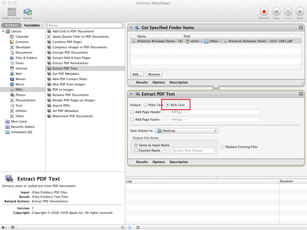
The key first step was provided by this tutorial on using the Automator program bundled with most Mac computers to extract Rich Text from PDFs. The workflow I created looked like this:

Screen shot of Automator workflow

Screen shot of Automator workflow

Extracting the text as "Rich Text" was the key. Running this workflow put an RTF file on my desktop that I then opened in Microsoft Word, which (I must now grudgingly admit) has some very useful features for a job like this. When I opened the file, for example, I noticed that all of the footnote text was a certain font size. I then used Word’s find and replace formatted text function to find and eliminate all text of that font size.

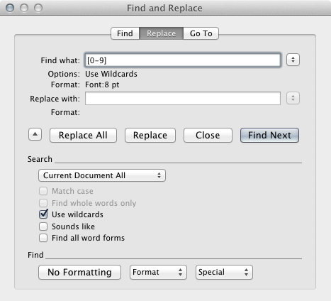
I used a similar technique to get rid of all the footnote reference numbers in the text, but in this case I had to be more specific because some of the text I wanted to preserve (like superscript "th," "st, and "nd" for ordinal numbers like "4th," "1st," and "2nd") was the same font size as the footnote markers. So I used Word’s native version of regular expressions (called wildcards) to find only numbers of that font size. In other words, the "Advanced Find and Replace" dialogue I used looked like this:

Word find and replace dialogue with wildcards

Word find and replace dialogue with wildcards

I used the same technique to eliminate the reference numbers leftover from the eliminated footnotes, which were all of an even smaller font size. Similar adjustments can be made by noticing that many of the ordinal suffixes mentioned earlier ("th," "st," and "nd") are "raised" or "lowered" by a certain number of points. You can see this by selecting those abbreviations and then opening the Font window in Word. Clicking on the "Advanced" tab will reveal whether the text has been lowered or raised. An advanced find and replace to change all text raised or lowered by specific points with text that is not raised or lowered fixed some, though not all, of these problems.

At this point I reached the limit of what I could do with the formatting find and replace features in Word, so I saved my document as a Plain Text file (with the UTF-8 encoding option checked to make things easier later on our Python parsing script), and then opened it up in a text editor. At this point I noticed that there were still some problems (though not as many!) in the text:

Houston, we have a problem

Houston, we have a problem

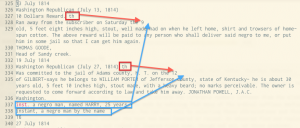
The main problem seems to arise in cases where there was a superscript ordinal suffix in the first line of an ad. As you can see, the "th" ends up getting booted up to the first line, and the remainder of the line gets booted down to the bottom of the page. Fortunately, there seems to be some pattern to this madness, a pattern susceptible to regular expressions. I also noticed that the orphaned line fragments following ordinals seem to always be moved to the bottom of the "page" right before the page number (in this case "16"). This made it possible to do a regex search for any lines ending in "th" (or "st" or "nd") followed by another line ending in a number, followed by a replacement that moves the suffix to where it should be. Though it took a while to manually confirm each of these replacements (I was worried about inadvertently destroying text), it wasn’t too hard to do.

A second regex search for page numbers allowed me to find all of the orphan fragments and manually move them to the lines where they should be (checking the master file from DRS in cases where it wasn’t clear which ad each fragment went with). The final step (which we already learned how to do in class) was to use a regular expression to remove all the year headers and page numbers from the file, as well as any blank lines. Franco’s drsparser script did the rest of the work of bursting the text file into individual ads and named the files using the provided metadata.

Team 1 Progress Report 3/31

Our task is to compare the Texas ads to those from Arkansas and Mississippi .  We will be utilizing a range of tools for this, many of which we have touched on in class.  We are looking at our work as a series of progressive tasks mining the ad content for deeper trends and information.

Our first task is to complete a close reading of the ads in question.  This will familiarize us with the material and provide grounds for categorizing key concepts, words, and phrases that we should search for.  By Wednesday, April 2nd, Alyssa will have done a close reading of the Austin Gazette ads and Daniel will have read the Texas Register ads from the overlapping years.  This will give a starting point of keywords and concepts we’re looking at to start the write up.

By April 7th, Daniel will have begun the text analysis of Texas and Arkansas ads with digital tools and the findings of the close readings.  He will share these with Alyssa, who will work on the close reading write-up due that day.

Our second task will then consist of utilizing these keywords and concepts to search the text with Voyant and TF-IDF.  We can look for trends and differences across states in the various results and visualizations we get from these.  We can also verify some of the categories by running the text through topic modeling, and searching those results for trends in Voyant as well.  Our future progress reports will include a commentary on how well these tools have worked for various purposes, for the benefit of future studies using these tools.

From this point, we plan to be flexible based on the findings of the text analysis.  Specific results might encourage further mining of the text for trends, or else might require us to go back to some of our earlier readings  for comparison or contrast of findings.  We can also at this point see if filtering the jailors’ ads from the text will change the language trends of the ads significantly, or if in fact the language of the different types of ads are highly similar.

GeoTeam Schedule

Monday, March 31st

Split up Arkansas and Mississippi corpus into individual ad files using drsparser.py – Aaron

Write python script placetagger.py to tag places using Pyner in a folder of text files and save the results – Aaron

Tuesday, April 1st

Run placetagger.py on Arkansas, Mississippi, and Texas (Gazette and Telegraph) corpus – Aaron

Run placetagger.py on Mississippi corpus – Kaitlyn

Start looking over required readings from earlier in the semester for more information about trends in runaway destinations and connections among Texas, Mississippi, and Arkansas. Do additional readings if necessary – Clare

Wednesday, April 2nd – Friday, April 4th

Clean up Named Entity Recognitions results – Aaron and Kaitlyn

  • Remove false positives
  • As thoroughly as possible given the magnitude of the collection, scan through tagged documents for any obvious false negatives
  • Tag each tagged location as a to or from, projected or real

Look over our data and outline the essay – Clare

Test drive Palladio and research other mapping options for displaying our place connections results – All

Saturday, April 5th – Sunday, April 6th

Analyze Named Entity Recognition results – All

If a lot of NER results:

  • Research geocoding APIs to parse our NER results and generate latitude/longitude coordinates for all named places – Aaron
  • Write script to generate coordinates for tagged locations and execute on our data – Aaron

Else:

  • Manually search for and store coordinates – Kaitlyn

Draft the close reading essay – Clare

Write progress update for course blog – Aaron and Kaitlyn

Monday, April 7th – Tuesday, April 8th

Decide on how we want to display our place connectedness results – All

  • How to display our results? Lines connecting the “to” coordinates (e.g. projected destination) and the “from” coordinates (e.g. coordinates of Houston for the Texas Register)? Something more individualized, at the ad-level? Collapse lines between cities or even states into single weighted lines by the number of that connection?
  • Building onto the first question, how to indicate direction: different line shapes/colors? For example, if there is a Texas ad that says their runaway probably went to his family in Arkansas, how to we differentiate that from an Arkansas jailor notice for a runaway slave saying he is from Texas? Is it important at all for us to make this distinction? If not, we might do better with a map in the form of an undirected graph.
  • How to separate projected runaway “to’s” (and guessed “from’s” for jailor’s notices, if ads like that exist) from actual “to’s” and “from’s”? Do we have much more of one type (real. vs guessed) — probably almost exclusively guessed locations?

Wednesday, April 9th – Friday, April 11th

Coordinate analysis and clean up – All

Re-assess rest of semester schedule in light of presentation format choices – All

Choose a mapping tool. Start building our map based on our decisions about to, from, projected, etc – All

Saturday, April 12th – Sunday, April 13th

Discuss our overall findings, and how our graphs and/or interactive tools share this information – All

Write and post progress report on course blog (by Monday) – All

Monday, April 14th – Wednesday, April 16th

Begin Methods page – Aaron and Kaitlyn

Begin Conclusions page, including followup questions and summary of findings – Clare

Finish our map and other graphics – All

Thursday, April 17th – Sunday, April 20th

Write and post progress report – All

Finish Methods page – Aaron and Kaitlyn

Finish Conclusions page – All

Monday, April 21st – Friday, April 25th

Finalize website pages – All

Throughout, Clare will re-work the essay in light of any new info.

Posting Ads to Twitter

Daniel’s question in class on Monday, about whether we were planning to release the ads we have found to the public, reminded me that we had earlier discussed the possibility of tweeting out our transcriptions with a link to the zoomed image in Portal of Texas History.

This tutorial suggests that may not be too difficult, especially now that we have a way to get all of our transcriptions out of our spreadsheets and into text files. It would be possible to write a script that reconstructs the URL to the page image from the title of our text files, and then tweets the first several words of the transcription with a link. That could be a way both of sharing our finds and of increasing interest in our larger project.

Is this something we would still be interested in doing? Thoughts?

Team Assignments

As discussed yesterday in class, we are going to split up into new teams to begin working on our final web project.

Both teams will contribute two things to the final project:

  • A webpage that contains an introduction to the question, a step-by-step section discussing different methods you tried to answer the question, and a summary of findings and questions for future research.
  • At least one non-narrative visualization illustrating some of the team’s findings.
  • A brief, traditional historical essay that answers the team’s question using a close reading of the available sources. These will be combined together on one page separate from the digital methods reports.

Your team should not only try the methods identified below to answer the question, but also reflect and report on whether these methods actually help us answer the question posed. You should also not take for granted that the corpora we have are already suitably prepared for the methods you want to try; your team may need to think through how to turn the transcriptions and metadata we’ve collected into datasets that are actually susceptible to the kinds of analysis you want to try.

Team 1

Alyssa and Daniel

Question

How similar were Texas ads to ads from the nearby states of Mississippi and Arkansas?

Method

Use text mining methods, such as word trends (in Voyant), TF-IDF, and topic modeling, to compare corpora from Texas, Mississippi and Arkansas.

Team 2

Aaron, Clare, and Kaitlyn

Question

Judging from runaway ads, how were Texas, Mississippi, Arkansas, and Louisiana connected geographically in the antebellum period?

Method

Use Named Entity Recognition to extract place names from the ad corpora and then try different methods (place count tables and graphs, Google maps, network graphs) to visualize how often places from one state were mentioned in another state’s ads.

Deadlines for Progress Reports

All progress reports from here on out will be due before class begins.

  • March 31: Report should include schedule for team’s tasks and work and initial delegation of tasks among team members
  • April 7: Report should include a draft of the "close reading" essay required for the final project, as well as update on other tasks
  • April 14 and 21: Report on progress toward final webpage

Got questions? Leave comments!

Update on TAPoR

After completing last week’s progress report, one of the questions we were left with is how the TAPoR Comparator calculates relative ratio. The documentation page does not specify where the relative count or the relative ratio come from, but a few trial calculations we able to lead us down the right path. We tested out numbers for “negro,” the most frequently occurring word in the Arkansas document from the Documenting Runaway Slaves Project project.

The results? The relative count equals the word count divided by the total number of words, so in this case, 920/80,690 for Arkansas, and 2,688/235,602 for Mississippi. Next, the relative ratio equals the Text 1 relative count divided by the Text 2 relative count, 0.0114/0.0114. Words that are relatively more frequent in Text 1 (AR) have a relative ratio value higher than 1, words that are relatively more frequent in Text 2 (MS) have a relative ratio value lower than 1, and words that are relatively equal have a value of 1. The relative ratio adjusts for document length and raw word counts to compare relative word frequencies. For example, even though “negro” has more than double the word count for Mississippi, the relative count for both AR and MS is ~0.0114. This places the relative ratio at 0.9994 – almost 1. (The reason this value is not exactly 1 is because the displayed relative counts get rounded off after the 4th decimal place. The relative counts for AR and MS are not actually precisely the same numbers down to the last decimal place).

So, Comparator balances the differences in document length between AR and MS to reveal that relatively, advertisements from the two states use the word “negro” with practically equal frequency. This sort of comparison could be useful for determining how language used to refer to the race of slaves does (or doesn’t) change across states. Similarly to TF-IDF, Comparator attempts to adjust for term frequency across documents to locate words that are more commonly occurring in one document compared to the rest of the corpus.

Now that we know how they both work, it would be interesting to compare our documents using both TAPoR’s Comparator and TF-IDF to see how the results differ. Here are the results for the word “negro” in Voyant’s TF-IDF option, recently added by Stefan Sinclair.
Again, AR and MS have very similar TF-IDF scores for the word “negro” despite MS’s raw word count being much higher.

You can view the raw word comparison output from TAPoR comparator at this webpage. You can also view the raw output from Voyant tools at this webpage.

Getting Ads from our Spreadsheets

Over the weekend I wrote up a script called txparser.py to get our Texas ads out of the Google Drive spreadsheet where we’ve been collecting them. To use the script, I first downloaded each sheet of our spreadsheet into a separate CSV (comma-separated value) file. (This is a text-based spreadsheet file format that can be easily opened in Microsoft Excel, by the way.) The script then iterates over the CSV files and generates a ZIP file containing each transcribed ad in a text file of its own.

Continue reading