Category Archives: Tools

Script for Counting Ads

Some of you expressed an interest in being able to quickly count all the ads in a folder and determine how many were published in a given year, decade, or month (to detect seasonal patterns across the year).

Here is a script that can do that. It is designed to work on Mac or Linux systems.

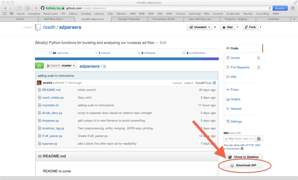
To use it, you should first download our adparsers repo by clicking on the "Download Zip" button on this page:

Download the adparsers repo as a zip

Download the adparsers repo as a zip

Unzip the downloaded file, and you should then have a directory that contains (among other things) the countads.sh script.

You should now copy the file to the directory that contains the ads you want to count. You can do this the drag-and-drop way, or you can use your terminal and the cp command. (If you forgot what that command does, revisit the Command Line bootcamp that was part of the MALLET homework. Once the script is in the directory, navigate to that directory in your terminal, and then run the command like this:

 ./countads.sh

If you get an error message, you may need to follow the instructions in the comments at the start of the script (which you can read on GitHub) to change the permissions. But if all goes well, you’ll see a printed breakdown of chronological counts. For example, when I run the script in the directory containing all our Mississippi ads, the script returns this:

TOTAL   1632 
     
DEC     ADS
1830s   1118
1840s   178
1850s   133
1860s   4
     
YEAR    ADS
1830    30
1831    54
1832    87
1833    68
1834    143
1835    157
1836    262
1837    226
1838    63
1839    28
1840    16
1841    16
1842    22
1843    33
1844    44
1845    25
1846    14
1847    1
1848    5
1849    2
1850    11
1851    17
1852    19
1853    15
1854    7
1855    9
1856    11
1857    23
1858    13
1859    8
1860    4
     
MONTH   ADS
1   100
2   89
3   103
4   130
5   160
6   161
7   188
8   150
9   150
10  149
11  146
12  86

If you choose, you can also "redirect" this output to a file, like this:

./countads.sh > filename.txt

Now you should be able to open filename.txt (which you can name whatever you want) in Microsoft Excel, and you’ll have a spreadsheet with all the numbers.

The script may seem to have limited value, but the key to its utility lies in first getting an interesting set of ads into a directory. That extends its usefulness. For example, if you wanted only to know the month distribution of ads in a particular year, you could first move all the ads from that year into a directory, and run the script from within it. You’d get lots of zeroes for all the years that you’re not interested in, but you would get the month breakdown that you are interested in. Depending on which ads you put in the directory that you are counting in, you can get a lot of useful data that can then be graphed or added into further calculations.

Getting Ads from our Spreadsheets

Over the weekend I wrote up a script called txparser.py to get our Texas ads out of the Google Drive spreadsheet where we’ve been collecting them. To use the script, I first downloaded each sheet of our spreadsheet into a separate CSV (comma-separated value) file. (This is a text-based spreadsheet file format that can be easily opened in Microsoft Excel, by the way.) The script then iterates over the CSV files and generates a ZIP file containing each transcribed ad in a text file of its own.

Continue reading

Measuring Document Similarity and Comparing Corpora

This past week, Alyssa and I have been looking at ways to quantify similarity of documents. We are doing this in the context of comparing Texas runaway slave ads to runaway slave ads from other states. Thanks to the meticulous work of Dr. Max Grivno and Dr. Douglas Chambers in the Documenting Runaway Slaves project at the Southern Miss Department of History, we have at our disposal a sizable set of transcribed runaway slave ads from Arkansas and Mississippi that we will be able to experiment with. Since the transcriptions are not in the individual-document format needed to measure similarity, Franco will be using regex to split those corpora into their component advertisements.

The common method to measure document similarity is taking the cosine similarity of TF-IDF (term frequency–inverse document frequency) scores for words in each pair of documents. You can read more about how it works and how to implement it in this post by Jana Vembunarayanan at the blog Seeking Similarity. Essentially, term frequency values for each token (unique word) in a document are obtained by counting the occurrences of a word within that document, then those values are normalized by the inverse document frequency (IDF). The IDF is the log of the ratio of the total number of documents to the number of documents containing that word. Multiplying the term frequency by the inverse document frequency thus weights the term by how common it is in the rest of corpus. Words that occur in high frequency in a specific document but rarely in the rest of the corpus achieve high TF-IDF scores, while words that occur in lower frequency in a specific document but commonly in the rest of the corpus achieve high TF-IDF scores.

Using cosine similarity with TF-IDF seems to be the accepted way to compute pairwise document similarity, and as to not reinvent the wheel, we will probably use that method. That said, some creativity is needed to compare corpora as a wheel, rather than just two documents. For example, which corpora are most similar: Texas’s and Arkansas’s, Arkansas’s and Mississippi’s, or Texas’s and Mississippi’s? We could compute an average similarity of all pairs of documents in each pair of corpora.

Just as a side-note, if we solve the problem of automatically transcribing individual Texas runaway ads, we could use cosine similarity and TF-IDF to locate duplicate ads. Runaway slave ads were often posted multiple times in a newspaper, sometimes with minor differences between each printing of the advertisement (for example, in reward amount). We could classify pairs of documents with a cosine similarity score greater than a specified threshold as duplicates.

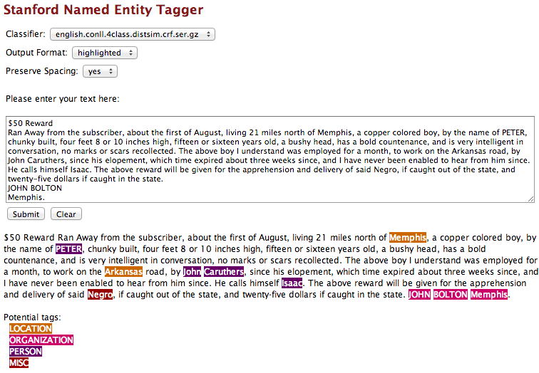
We could also use Named Entity Recognition to measure the similarity of corpora in terms of place-connectedness. Named Entity Recognition is a tool to discover and label words as places, names, companies, etc. Names might not be too helpful since, as far as I have been able to tell, slaves were usually identified just by a first name, but it would be interesting to see which corpora reference locations corresponding to another state. For example, there might be a runaway slave ad listed in the Telegraph and Texas Register in which a slave was thought to be heading northeast towards Little Rock, where he/she has family. The Arkansas corpus would undoubtedly have many ads with the term Little Rock. If there were a significant number of ads in Texas mentioning Arkansas places, or vice-versa, this is information we would want to capture to measure how connected the Texas and Arkansas corpora are.

Demo run of Stanford's Named Entity Tagger on an Arkansas runaway slave ad

A simple way we could quantify this measure of place-connectedness would start with a Named Entity Recognition list of tokens and what type of named entity they are (if any). Then we would iterate through all tokens and, if the token represents a location in another state in the corpus (perhaps the Google Maps API could be used?), increment the place-connectedness score for that pair of states.

We also explored other tools that can be used to compare text documents. In class, we have already looked at Voyant Tools, and now have been looking at other types of publicly available tools that can be used to compare documents side by side. TAPoR, is a useful resource that lets you browse and discover a huge collection of text analysis tools from around the web. It contains tools for comparing documents as well as for other kinds of text analysis. As we move forward with our project, TAPoR could definitely be a great resource for finding and experimenting with different tools that can be applied to our collection of runaway slave ads.

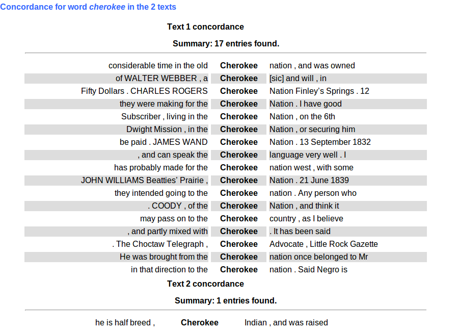
TAPoR provides a tool from TAPoRware called Comparator that analyzes two documents side by side to compare word counts and word ratios. We tested this tool on the Arkansas and Mississippi runaway advertisement collections. This sample comparison already yields interesting results, and gives an idea of how we could use word ratios to raise questions about runaway slave patterns across states.

These screenshots show a test run of the ads through the TAPoR comparator; the Arkansas ads are Text 1 and the Mississippi ads are Text 2. This comparison reveals that the words “Cherokee” and “Indians” have a high relative frequency for the Arkansas corpus, perhaps suggesting a higher rate of interaction between runaway slaves and Native Americans in Arkansas than in Mississippi. Click on a word of interest to get a snippet of the word in context. Upon looking into the full text of ads containing the word “Cherokee”, we find descriptions of slaves running away to live in the Cherokee nation, or running away in the company of Native Americans, slaves that were part Cherokee and could speak the language, or even one of a slave formerly being owned by a Cherokee.

However, after digging into the word ratios a little deeper, it turns out that uses of the word “Choctaw” and “Indian” are about even for Arkansas and Mississippi, so the states in the end may have similar patterns of runaway interaction with Native Americans. Nevertheless, this test of the Comparator gives us an idea of the sorts of questions it could help raise and answer when comparing advertisements. For example, many of us were curious if Texas runaway slaves ran away to Mexico or ran away with Mexicans. We could use this tool to look at ratios of the words “Mexico” or “Mexican” in Texas in comparison to other states.

Some Text Mining Resources

Today in class I briefly mentioned TF-IDF (Term Frequency-Inverse Document Frequency) as a possible way for us to identify "give away" words that might appear more frequently in a particular document. Here are some introductory explanations of the method:

And here’s a cool visualization experiment using TF-IDF made by Tim Sherratt, who also made the Real Face of White Australia and Headline Roulette sites shown in class today.

I also mentioned Named Entity Recognition in class; this is the same library used by the Rezo Viz tool that Daniel and Alyssa showed us in their Voyant Tools presentation. It may be possible for us simply to use Voyant as an interface for NER and export a list of place and person names from our ads, but we need to look into this further.

Slides from Tool Presentations

Thanks for the great job that you all did on your presentations about digital tools that might be helpful for our project with runaway slave ads! I’m posting here the slides that were shown in class so that we can reference them. Click the image to get the whole PDF.

First, Alyssa and Daniel talked with us about Voyant Tools:

Clare and Kaitlyn talked about using Google Maps and Google Fusion Tables, together with Social Explorer:

Thanks for sharing!

Discovering Runaway Slave Ads

These last few days, Franco and I have been developing a way to detect runaway slave ads in images of 19th centuries newspapers. The Portal to Texas History has digitized copies of thousands of issues of Texas newspapers and is a source waiting to be explored for runaway slave ads. For example, a search for “runaway negro” in the full-text (OCR transcriptions) of their collection yields 7,159(!) results. Clearly, that number is too high to accommodate manual perusal of all possible matches.

Fugitive Slave IconThus, we have been thinking about ways to automate the process. Under the suggestion of Dr. McDaniel, we decided to use OpenCV, a popular open source computer vision library, to conduct object recognition for the classic runaway slave icon. You know, this one:

(In newspapers, from what I have seen, it usually appeared much smaller and simplified, as shown here).

OpenCV has a tool called Cascade Classifier Training that builds an XML file that can be used to detect objects. It requires a set of positive samples, images that contain the chosen object, and negative samples, images that do not contain the object but are of similar context. It works best with a large dataset of positive samples, and to generate that it provides a function called “createsamples” that takes an image and applies transformations to it, such as adjustments in intensity, rotations, color inversions, and more to make altered versions. Once the cascade has been trained, it can be used to efficiently detect and locate the desired object in other images.

So, the first order of business in preparing to do object recognition was to collect a set of runaway slave icons. I downloaded ~35 newspaper page images containing the icon and cropped the images to only contain the icon visible. The tutorials [1, 2, 3 ..others] I read suggested that for best results the positive images (images of the object to be detected) should all be the same aspect ratio. For simplicity, I made sure all my images were 60x64px.

Next I generated a set of negative (background) images that were from newspaper images that did not have the runaway icon. These had to be the same size as the positive images. I read that a large data set was especially needed for the negatives, so I wrote a simple script to crop newspaper page images into a series of individual 60×64 pics. For anyone curious, here’s a gist of the code. Sample background imageA typical image looked something like this.

Negative sample for training the HAAR cascadeAfter running the script on several images, I ended up with ~1600 negative images to use in training the cascade classifier. I supplemented that with some manually-cropped pics of common icons such as the one that appears to the left.
Next I used the find command in terminal to output text files containing a list of all the positive and all the negative images. Then, I created the “sample,” a binary file that contains all the positive images that is required by the cascade trainer (opencv_traincascade). Like I mentioned, usually in creating the sample, transforming settings are specified to multiply the amount of data available to train the cascade. I figured that the runaway icon would always appear upright, and I made sure my positive images set contained icons of varying clarity, so I just ran opencv_createsamples without any distortions.

Finally, I had all I needed to train the cascade. I ran the following command in Terminal:
opencv_traincascade -data classifier -vec samples/samples.vec -bg negatives.txt -numStages 6 -minHitRate 0.95 -numPos 27 -numNeg 1613 -w 60 -h 64 -precalcValBufSize 512 -precalcIdxBufSize 256

Opencv_traincascade is the program to be run. The value for data is the name of the folder to store the resulting cascade file in. The value for vec is the path to the samples vector file. The value for bg is the name of the file containing paths to each negative image. numStages I am not entirely sure so I just picked 6 since I didn’t want the training to run for days as others have experienced. minHitRate dictates the accuracy. numPos I still don’t quite understand, but I chose ~80% of the number of positive images to ensure no errors would result. numNeg is the number of negative images. Then there’s width, height, and some settings specifying how much RAM the program can hog up.

I had high hopes, but after 30 minutes of fans-blaring CPU use the program quit with the error, “Required leaf false alarm rate achieved. Branch training terminated.” I need to do more research to figure out why it didn’t work, but an initial search told me that the number of positive samples I used may not be enough. Joy..

Next Steps:

  • Play around with OpenCV some more to try to get a functional cascade. Maybe enlist the help of stackoverflow or reddit.
  • Rethink whether object recognition is the best way to maximize runaway slave ad discovery. While a lot of ads did use the icon, perhaps a larger number did not. For newspapers with digital transcriptions, text-based analysis would surely provide better results.
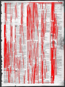
  • If we can’t get a working cascade to do object recognition, revisit newspaper decomposition. Franco and I tried using Hough Line Transforms through OpenCV to detect lines separating newspaper articles, but to no avail. Its promise is marked up images like the Sudoku board shown below. To the right of it is our “success.” The theory is that if we could detect the dividing lines in newspapers, we could crop the pages into individual articles, run OCR on each article, and then do text-analysis to discover runaway ads. It is no easy feat, though, as these [1, 2] research articles demonstrate.
  • I was able to improve our results by limiting detected lines to those with approximately horizontal or vertical slopes, since those are the only ones we are interested in newspapers, but it is clear we need to tweak the script or enlist a better system.

    Marked up Sudoku board using Hough Line Transform

    Sudoku hough line transform

    Hough Line Transform output

    Best we can do so far..

    If you have any tips or feedback, feel free to contact Franco (@FrancoBettati31) or me (@brawnstein) on Twitter, or leave a comment below. Thanks!

Using Voyant Tools for Runaway Ads

I’ve been using the site Voyant Tools to look at the text content of runaway ads.
In a nutshell, the site pulls all the words, and finds their frequencies and trends.  It displays them in a variety of ways, which I’ll show with its analysis of 550 pages of Mississippi slave ads.

Without screenshots, you can view the results through this link (one feature is the enabled url and unique ID for data sets, which allows re-linking and comparing between documents).

Features include Cirrus- a basic word cloud, numerical data for the appearances of words in the corpus, the option to see each appearance in context, and Trends- a tool that visually maps out the relative frequency of the word throughout the course of the document.

This last tool is the most interesting to me, as in chronologically ordered ad sets, it gives you an immediate look at the relative usage of the term over time.  For example, the use of 1836 has one remarkable spike in usage over the course of several decades… We can use this to track usage of racial descriptive terms over time, or similar word-based information.

Through the incorporation of numerous corpuses of information, we can also compare word usage in different states and areas.  I can see how this will be helpful in the future in answering some of our questions regarding how Texas runaways and situations were different from those in the rest of the south.

HW#5: Thoughts and Progress on Voyant

For the group presentations, I’ve been working with the tool Voyant, which does text analysis on one or more documents. Among its tools, it generates a word cloud of most frequent words, generates graphs of word frequency across the corpus, and lets you compare multiple documents. Once you have a text uploaded, you can play around a lot within the Voyant “skin”, opening and closing different tools, or clicking on a particular word to see trends for that word specifically. It’s also possible to generate a link to the skin that can then be shared with others, allowing them to then play around with the data on their own. I think this interactive feature could potentially be really useful, since it lets anyone who is curious take a look at the data and track key words in pursuit of whatever questions they might be interested in.

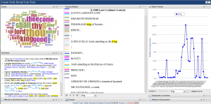
Just as an example of what using the Voyant tools looks like, this screenshot shows Shakespeare’s works (Voyant’s sample corpus).

Right now I have the word “king” selected, allowing me to see specific information about the word such as where in the corpus the word appears, frequencies of the word over time, and the word in context.

To apply Voyant specifically to runaway slave ads, Daniel and I looked at transcribed documents of runaway slave ads from Mississippi and Arkansas (PDF’s available from Documenting Runaway Slaves Project). I looked at the Arkansas ads, splitting the corpus up in two different ways. First, I split the document up by decade and then a single document of the ads from 1820-1865. (note: to turn off common stop words such as “and” “the”, click the gear icon and choose English for list of stop words) Splitting the ads up by decade could potentially make it easier to track changes over time, although since the original document was already ordered chronologically this is also possible to do with the single document. Another possibility we talked about in class is splitting up runaway ads into individual documents, making it possible to compare specific ads, rather than time clumps.

During class, Daniel and I combined the Arkansas and Mississippi documents to do a side-by-side comparison of the two states. Not surprisingly, “Arkansas” is a distinctive word in the Arkansas documents, but with other words such as “sheriff” or “committed” it could be interesting to dig down deeper and figure out why those differences exist. Are these merely linguistic/word choice differences, or do they indicate a difference in runaway patterns? These are the sorts of questions which Voyant raises, but can also help answer, with tools such as keywords in context.

I was interested in comparing the work we’d already done on Mississippi and Arkansas to some of the Texas ads we’ve collected in the Telegraph and Texas Register. I transcribed Texas ads from 1837 (excluding reprints) and compared that with Mississippi and Arkansas ads from 1837. The sample from Texas is small, so I would be hesitant to draw grand conclusions from this comparison, but it’s a good place to start addressing the questions many of us were interested in about what difference Texas makes (if any) in runaway patterns. Here are the results of all three states for 1837. Looking forward, I’m interested in looking at these results more closely to see if they raise interesting questions regarding Texas. This can help us answer questions about whether or not it’s worthwhile to continue transcribing Texas ads (and if so, how many), and how to split up the data (by year, by individual advertisement?).

The main downside to using Voyant so far is the same issue we ran into with Mallett: the Telegraph and Texas Register advertisements are not available individually in text format. This is not so much a limitation with Voyant itself as it is with the medium of primary source documents we are working with. It does seem at this point that Voyant could be a useful tool, but if we as a class decide to use Voyant for our project in the future, we’ll have to think of ways to get around that obstacle.

Group Presentations

In the next two weeks of class, we will divide our labor so that we can learn about some different kinds of digital tools that might help us answer (or more effectively present our answers) to our questions about slavery and runaway slave ads in Texas.

You will work with a partner to work through some tutorials (much like you did for Homework #3), and then talk with your partner about how this tool (or others like it) might be useful for our class. Your final task will then be to report back to the class on what you have done with an oral presentation that gives your classmates a sense of what the tool can do and what it might do for us.

Continue reading

Homework #3: Using and Understanding MALLET

If you prefer, you may download this assignment in PDF form.

For our January 31 class, you read several articles about using a method called "topic modeling" to "read" texts algorithmically. In this homework assignment, you will have a chance to use MALLET, a topic modeling software package, yourself and then write a reflection on your experience that applies what you have learned to our class project.

Before You Begin

This assignment will require you to use the command line on your computer. I recommend that before you begin, you review some of the material on this that we covered in class on Friday.

If you have a Mac or Linux machine, the Command Line Bootcamp from the Scholars’ Lab at the University of Virginia is a useful place to begin, and it is aimed at humanities students and scholars. If you have a Windows machine, here is a basic introduction to the DOS prompt.

Regardless of your machine, there are three main things you will need to be able to do in this assignment from the command line, so make sure you understand how to do each of them:

  • See what directory you are currently in.
  • Change directories.
  • List the contents of the current directory.
  • See inside the contents of a file.

You may also want to know how to clear your terminal screen if it becomes too crowded with text. You can do this with the command cls at the Windows command prompt and the command clear at the Unix/Mac command line. (Even after clearing the screen, you should be able to scroll up in your terminal windows to see what you’ve done in the past.)

Objectives

  1. To gain a basic familiarity with the command line.
  2. To install and use MALLET with the sample data included in the package.
  3. To reflect on the uses and limitations of topic modeling in historical research.
  4. To gain experience and confidence in following a detailed tutorial for an unfamiliar tool.

Requirements

There are both technical and non-technical requirements for this assignment, but the two parts are separable. I recommend that you attempt the technical part first since it will probably take longer, but if you get stuck, you should be able to answer the questions in the non-technical part before completing the techy stuff.

Technical Requirements

Complete the tutorial on Getting Started with Topic Modeling and MALLET at the Programming Historian, which will show you how to install MALLET and then use it on the sample documents included with the package.

This requirement will be completed when you tweet two screenshots of your work to the course hashtag #ricedh. More specifically:

  • One screenshot should, like Figure 8 in the tutorial, show the output of a train-topics command on the sample data set discussed in the tutorial, but should show that you generated 15 topics instead of the default 10.
  • One screenshot should, like Figure 10 in the tutorial, show a screenshot of the tutorial_composition.txt file generated by your 15-topic model opened in Excel. (If you don’t have Excel installed on your computer, you can also satisfy this requirement by creating a GitHub Gist containing the contents of your tutorial_composition.txt file and tweeting the link to the Gist instead.)

If you are not familiar with how to take screenshots on your computer, do some Googling to find out the answer, or ask on Twitter for help. You will also need to learn how to post photos on Twitter.

Non-Technical Requirements

After reading the Friday texts about topic modeling and trying out MALLET yourself, you should be able to figure out answers to the following two questions:

  1. Suppose we wanted to create a topic model of the runaway slave ads we have collected on our Google Spreadsheet. What first steps would we have to take to get from our spreadsheet of permalinks to a *.mallet file that we could train topics on?
  2. In his Mining the Dispatch project, Robert K. Nelson used MALLET to find articles that were likely to be fugitive slave ads in a large corpus of digitized newspapers. What feature(s) of the Portal to Texas History would have prevented us from using the same method to discover ads in the Telegraph and Texas Register? Be as specific and thorough as possible. (Here’s a hint: do some searching for keywords in the Telegraph and Texas Register on the Portal, and notice what kinds of results you get back. Does the kind of result returned by a keyword search tell you something about the way that the underlying text documents in the Portal are stored and separated from each other?)

Write up an email to me answering both of these questions. You should be able to answer them with just a few sentences in each case—no more than two good-sized paragraphs should do the job.

Summary and Evaluation

Successful completion of this assignment will include:

  • Two screenshots posted to Twitter to satisfy the technical requirements.
  • An email to me answering the two non-technical questions.

Because this assignment has several, separable parts, I will divide up the points for the assignment this way when evaluating your homework: two points for each screenshot, and three points for each answer in the email.

Help! I’m Stuck!

There is a good possibility you’ll encounter technical difficulties when doing this assignment. Don’t fret or bang your head against the wall all weekend if you are getting an error message that is not mentioned in the tutorial, or if you are having trouble getting the same results shown in the tutorial. Instead, get help!

You can always take to Twitter if you need help. If you are getting error messages in your terminal that are longer than 140-characters or difficult to explain, you can also use a Gist, as you did in the first homework, to get help. Copy and paste the strange output of your terminal into a Gist, putting an explanation of what produced it in the Gist "description," and then tweet the URL to that Gist to our course hashtag to see if I or another student can help. (And remember, helping out other students is a way to score well on the Team Participation part of your grade.)

Remember, though, the academic integrity policies for the course. Do not get someone else to do the work for you and be sure to acknowledge any pointers or technical assistance you received—in this case by noting it in your email to me.